Options Tab Right Panel
The right hand side panel of the Options tab allows you to turn the 6 main plot types on and off, and to change the settings for each group.
Spectra and Time Waveform Plots
The figure below shows the first few rows of the right hand panel of the options tab. The first row of check boxes allows you to turn on or off the 6 main plot types, which are:
- Time waveform of raw data (eg acceleration or noise)
- FFT of raw data
- Time waveform of integrated data (eg velocity data from acceleration)
- FFT of integrated data
- Time waveform of twice integrated data (eg displacement data from acceleration)
- FFT of twice integrated data
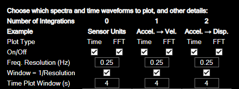
Frequency Resolution and Window Length
The next three rows show the frequency (bin) resolution for ffts, the time waveform duration used in analysis mode, and a button to link these. If they are linked, the frequency resolution will be the inverse of the time waveform duration, and the data shown in the time waveform plot will be the data that is used to calculate the FFT (see FFT Setup for a detailed explanation). In analysis mode, all of the time waveform data is shown, however you can still show the time window for the current FFT by disabling the peak hold and average spectra and turning on Plot Zoomed Time.
Option Grouping
The six columns below this contain (in a rough sense) the options for each of these six plot types. By default, if you turn one of these plot types on, it will be enabled for all acceleration channels (with units of g), or all channels in the case of raw data. You can turn off individual channels on the setup tab. Any options that are not currently available (for example because you are in analysis or acquisition mode) will be greyed out and inactive.
The figure below shows 3 copies of the entire right panel, showing how the options are grouped:
- Red: Raw data.
- Green: integrated data
- Blue: twice integrated data
- Yellow: time waveform plot options
- Purple: FFT plot options.
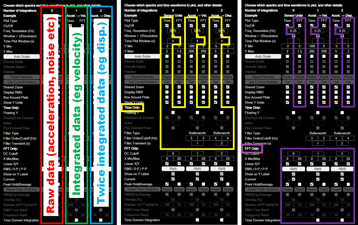
Detailed information on each option is provided below.
Common Options
On/Off: Turns the six plot types on or off for all channels.
Freq. Resolution (Hz): Bin resolution. The frequency offset between neighbouring data points on the FFT.
Window = 1/Resolution: Link the frequency resolution to the time waveform plot duration in acquisition mode, or to the zoomed time plot duration in analysis mode (if peak hold and average is turned off).
Time Plot Window (s): Time waveform plot duration in acquisition mode.
Y Min/Y Max: Y scale for each plot type. This can be over-ridden (increased) by auto scale.
Auto Scale: Automatically increase Y axis scaling.
Shared Scale: All plots of same type have same Y axis scale.
Smooth Adjust: Auto scale in very small steps
Ratchet: Do not reduce scale automatically, only increase it.
Reset Ratchets: Return to nominal Y scale specified above.
Get Current Scaling: Update the specified scale with the current scale.
Shared Zoom: To be included in next release. This is for zooming with the mouse.
Display RMS: Display text in the top left corner of each plot showing the overall RMS level.
Box Around Plots: Draw a box around the plots.
Show Y Units: Shows Ch 1 (mm/s) instead of just Ch 1. We advise against turning this off, as the amplitude is then ambiguous, however it may be convenient in situations where you have a lot of plots on one tab and the Y axis labels get too crowded and start to overlap.
Time Waveform Options
Floating Y: Y axis is not centred on zero.
Display/Link Cursors: Analysis mode only. Shows a cursor on the time waveform plot corresponding to the centre of the window used for the FFT.
Index: Time waveform data point (sample number) associated with cursor. Keep a record of this if you may want to reproduce your FFT.
Plot Zoomed Time: Analysis mode only. Shows a zoomed time waveform plot corresponding to the input data for the FFT. If peak hold or average is enabled, this plot spans all time windows used.
Filter Type: High pass filter type for time domain integration. Currently only Butterworth is available.
Filter Order/Cutoff (Hz): The number on the left in each pair is the filter order, and the number on the right is the cutoff in Hz. For the high pass filter for time domain integration.
Filter Transient (s): Discard data at the start of the integrated signal associated with filter ringing.
FFT Options
DC Cutoff: Discard the data below this frequency (in Hz) in the FFT. Often used for integrated data where low frequency noise is magnified.
X Min/Max: X axis limits.
Linear X/Y: Turn off the get a log scale on the X axis (left checkbox in each pair) or Y axis (right checkbox).
RMS / 0-P / P-P: Use Root Mean Square, zero to peak or peak to peak scaling. 0-P multiples FFT by the square root of 2. P-P amplitude is double the 0-P amplitude.
Show on Y Label: Show RMS / 0-P / P-P on Y axis label. We advise against turning this off, as the amplitude is then ambiguous, however it may be convenient in situations where you have a lot of plots on one tab and the Y axis labels get too crowded and start to overlap.
Current: Turns on current FFT. At least one of current, peak hold or average must be selected if the FFT option is on.
Peak Hold/Average: The left check box in each pair turns on the peak hold spectrum. The right check box turns on the average spectrum.
Reset Peak Hold/Avg: Acquisition mode only. Sets the peak hold plot to the current FFT.
RMS/Exp Average: Only used when average FFT is turned on. Both disabled: use a linear average. The left check box in each pair enables RMS averaging instead of linear. The right check box enables an exponentially decaying average, and can be used with both the linear and RMS option.
Overlap (%): For peak hold and average plots. 0% overlaps means one time window starts where the previous one ends. Negative numbers are allowed. -100% for example discards a full tie window between subsequent FFT windows. In acquisition mode, an approximate overlap is used for the average FFT, and the overlap is ignored for the peak hold FFT. The peak hold is updated as rapidly as the processor speed allows in acquisition mode, however this would cause certain time periods to be over-represented in an average spectrum.
Number of FFTs/Half N: Number of FFTs (right number from each pair) is only used in analysis mode, for the peak hold and average spectra. Half N (left number from each pair) is used for exponential averaging. Roughly speaking, if Half N is set to 10, the influence of the 10th most recent spectrum is half that of the most recent spectrum. Think of it as the half life in terms of number of spectra acquired.
RMS From Band: If RMS display is turned on (the added text in the top left corner of the plot, not the RMS/0-P/P-P option), calculate it from a section of the FFT defined below, rather than the whole FFT.
Frequency Band: Calculate the RMS between the frequencies defined by each pair of numbers (Xmin on the left of each pair, Xmax on the right).
Time Domain Integration: By default, all spectra are obtained from raw data and, if required, integrated in the time domain. Use this option if you want to use integrated time waveform data instead. It is close to the same answer. The main difference is that the integrated time waveform data is influenced by the high pass filter. This option is more computationally intensive, unless you have turned on the integrated time waveform plot, and are not calculating spectra from raw data for any other plots. If you are not plotting the integrated time waveform data, it is better to leave this option off and use the DC cutoff to remove any low frequency noise from the integrated spectrum.